1 Units, Vectors, and Scalar Quantities
1.1 SI Units
The course adopts the Système International (SI) of units. The base units most relevant to mechanics are:
| Quantity | Unit | Symbol |
|---|---|---|
| Mass | kilogram | kg |
| Length | metre | m |
| Time | second | s |
| Force | newton | N |
| Energy / Work | joule | J |
| Power | watt | W |
| Pressure / Stress | pascal | Pa |
Derived units follow from these. For example:
\[1 \text{ N} = 1 \text{ kg·m/s}^2 \qquad 1 \text{ Pa} = 1 \text{ N/m}^2 \qquad 1 \text{ J} = 1 \text{ N·m}\]
1.2 Scalar and Vector Quantities
Scalar quantities have magnitude only and obey ordinary arithmetic:
- Examples: mass, speed, temperature
Vector quantities have both magnitude and direction and must be combined using vector algebra:
- Examples: force, velocity, acceleration, momentum
A vector is represented graphically as an arrow — its length denotes magnitude, its orientation denotes direction.
1.3 Vector Addition
1.3.1 Triangle Rule
Two vectors \(\mathbf{A}\) and \(\mathbf{B}\) are added tip-to-tail; the resultant \(\mathbf{R}\) closes the triangle:
\[\mathbf{R} = \mathbf{A} + \mathbf{B}\]
1.3.2 Parallelogram Rule
Both vectors are drawn from the same point; the resultant is the diagonal of the parallelogram they form.
1.3.3 Polygon Rule
For more than two vectors, they are placed tip-to-tail in sequence; the resultant closes the polygon from the tail of the first to the tip of the last.
1.4 Vector Subtraction
Subtracting \(\mathbf{B}\) from \(\mathbf{A}\) is equivalent to adding the negative of \(\mathbf{B}\):
\[\mathbf{R} = \mathbf{A} - \mathbf{B} = \mathbf{A} + (-\mathbf{B})\]
1.5 Resolution of Vectors
Any vector \(\mathbf{F}\) can be resolved into two perpendicular components. For a vector at angle \(\theta\) to the horizontal:
\[F_x = F\cos\theta\] \[F_y = F\sin\theta\]
This is the most widely used technique in the book — resolving all forces into horizontal and vertical components before applying equilibrium conditions.
1.6 Resultant of Several Vectors
To find the resultant of a system of vectors analytically:
- Resolve each vector into \(x\) and \(y\) components
- Sum all components in each direction:
\[\Sigma F_x = F_{1x} + F_{2x} + \cdots \qquad \Sigma F_y = F_{1y} + F_{2y} + \cdots\]
- Find the magnitude of the resultant:
\[R = \sqrt{(\Sigma F_x)^2 + (\Sigma F_y)^2}\]
- Find the direction:
\[\theta = \arctan\left(\frac{\Sigma F_y}{\Sigma F_x}\right)\]
1.7 The Laws of Sines and Cosines
For cases involving triangles of vectors, these laws provide an analytical alternative to graphical methods.
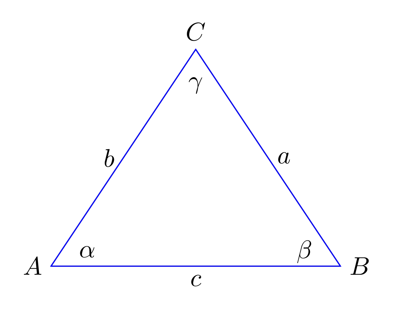
Sine rule:
\[\frac{a}{\sin \alpha} = \frac{b}{\sin \beta} = \frac{c}{\sin \gamma}\]
Cosine rule:
\[c^2 = a^2 + b^2 - 2ab\cos \gamma\]
1.8 Summary of Equations
| Concept | Equation |
|---|---|
| Horizontal component | \(F_x = F\cos\theta\) |
| Vertical component | \(F_y = F\sin\theta\) |
| Resultant magnitude | \(R = \sqrt{(\Sigma F_x)^2 + (\Sigma F_y)^2}\) |
| Resultant direction | \(\theta = \arctan(\Sigma F_y / \Sigma F_x)\) |
| Cosine rule | \(c^2 = a^2 + b^2 - 2ab\cos C\) |